####################################################################################################
#r#
#r# ========================
#r# Fast Fourier Transform
#r# ========================
#r#
#r# This example shows how to compute a FFT of a signal using the scipy Scientific Python package.
#r#
####################################################################################################
import numpy as np
from scipy import signal
from scipy.fftpack import fft
import matplotlib.pyplot as plt
####################################################################################################
#r#
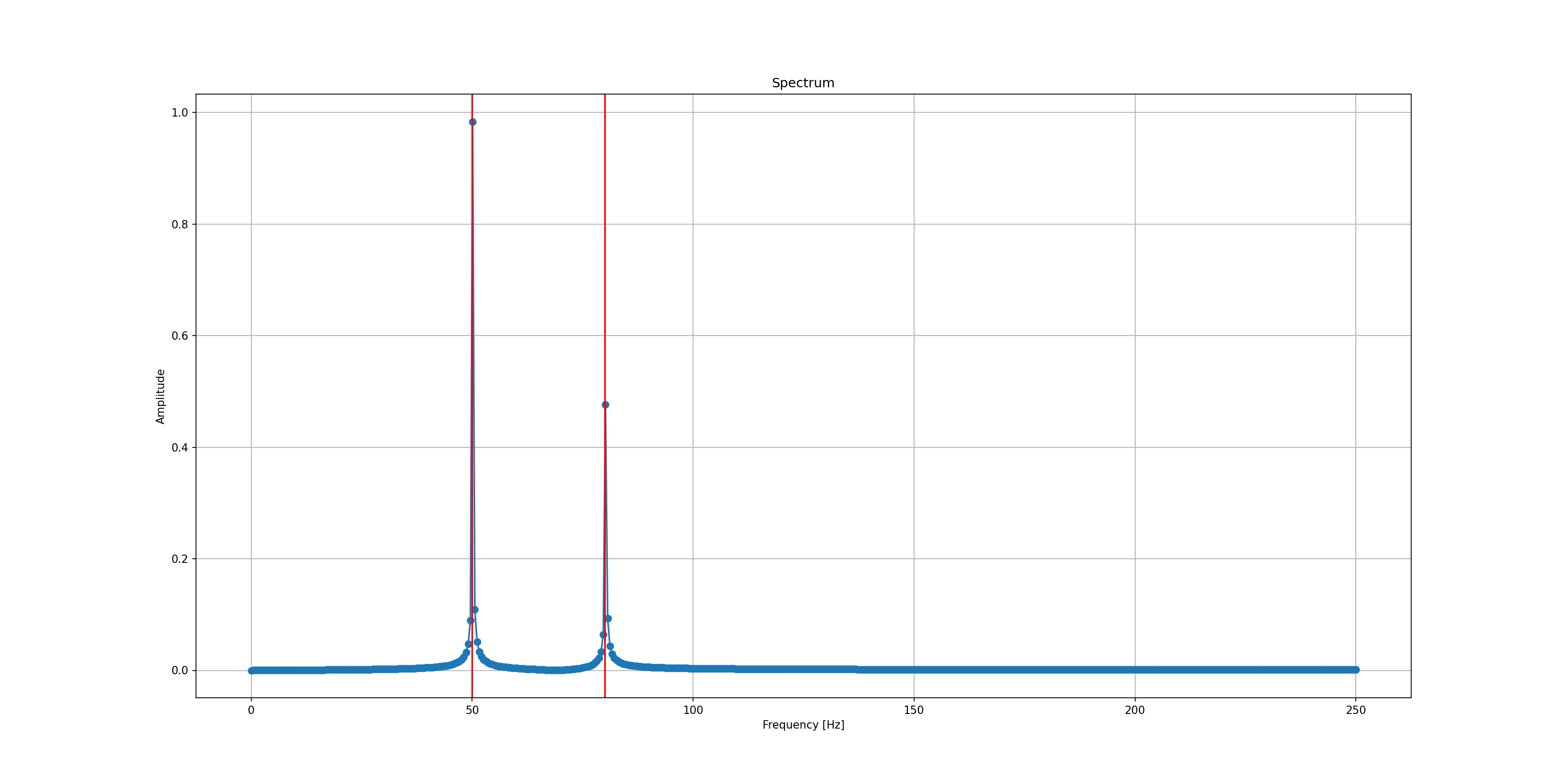
#r# We will first compute the spectrum of the sum of two sinusoidal waveforms.
#r#
N = 1000 # number of sample points
dt = 1. / 500 # sample spacing
frequency1 = 50.
frequency2 = 80.
t = np.linspace(0.0, N*dt, N)
y = np.sin(2*np.pi * frequency1 * t) + .5 * np.sin(2*np.pi * frequency2 * t)
yf = fft(y)
tf = np.linspace(.0, 1./(2.*dt), N//2)
spectrum = 2./N * np.abs(yf[0:N//2])
figure1, ax = plt.subplots(figsize=(20, 10))
ax.plot(tf, spectrum, 'o-')
ax.grid()
for frequency in frequency1, frequency2:
ax.axvline(x=frequency, color='red')
ax.set_title('Spectrum')
ax.set_xlabel('Frequency [Hz]')
ax.set_ylabel('Amplitude')
#f# save_figure('figure1', 'fft-sum-of-sin.png')
####################################################################################################
#r#
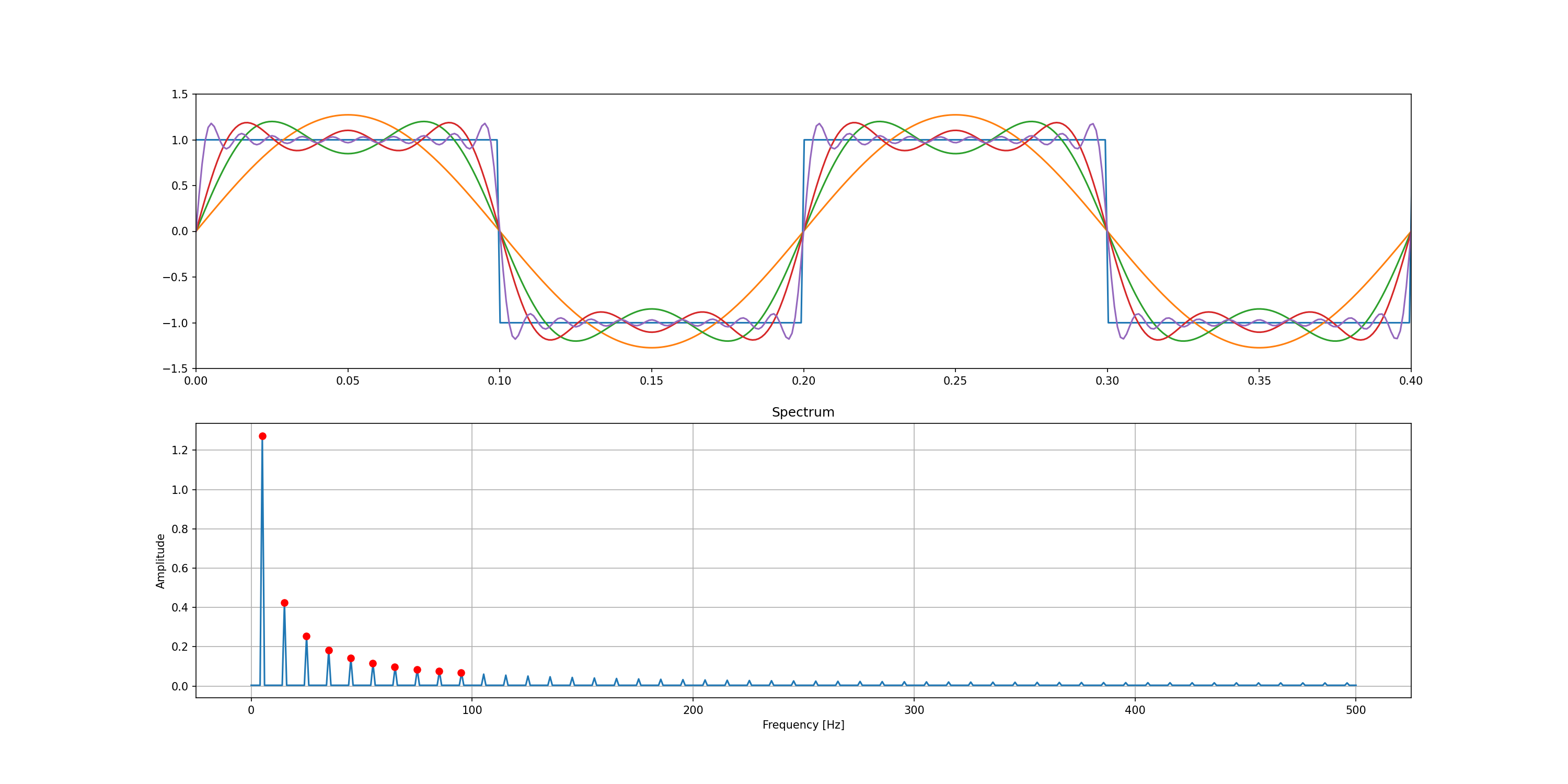
#r# Now we will compute the spectrum of a square waveform.
#r#
#r# The Fourier series is given by:
#r#
#r# .. math::
#r#
#r# \frac{4}{\pi} \sum_{n=1, 3, 5, \ldots}^{\inf} \frac{1}{n} \sin(n 2\pi f t)
#r#
N = 1000 # number of sample points
dt = 1. / 1000 # sample spacing
frequency = 5.
t = np.linspace(.0, N*dt, N)
y = signal.square(2*np.pi*frequency*t)
figure2, (ax1, ax2) = plt.subplots(2, figsize=(20, 10))
ax1.plot(t, y)
y_sum = None
for n in range(1, 20, 2):
yn = 4/(np.pi*n)*np.sin((2*np.pi*n*frequency*t))
if y_sum is None:
y_sum = yn
else:
y_sum += yn
if n in (1, 3, 5):
ax1.plot(t, y_sum)
ax1.plot(t, y_sum)
ax1.set_xlim(0, 2/frequency)
ax1.set_ylim(-1.5, 1.5)
yf = fft(y)
tf = np.linspace(.0, 1./(2.*dt), N//2)
spectrum = 2./N * np.abs(yf[0:N//2])
ax2.plot(tf, spectrum)
n = np.arange(1, 20, 2)
ax2.plot(n*frequency, 4/(np.pi*n), 'o', color='red')
ax2.grid()
ax2.set_title('Spectrum')
ax2.set_xlabel('Frequency [Hz]')
ax2.set_ylabel('Amplitude')
#f# save_figure('figure2', 'fft-square-waveform.png')
####################################################################################################
plt.show()
8.3.1. Fast Fourier Transform
This example shows how to compute a FFT of a signal using the scipy Scientific Python package.
import numpy as np

from scipy import signal
from scipy.fftpack import fft

import matplotlib.pyplot as plt
We will first compute the spectrum of the sum of two sinusoidal waveforms.
N = 1000 # number of sample points
dt = 1. / 500 # sample spacing

frequency1 = 50.
frequency2 = 80.

t = np.linspace(0.0, N*dt, N)
y = np.sin(2*np.pi * frequency1 * t) + .5 * np.sin(2*np.pi * frequency2 * t)

yf = fft(y)
tf = np.linspace(.0, 1./(2.*dt), N//2)
spectrum = 2./N * np.abs(yf[0:N//2])

figure1, ax = plt.subplots(figsize=(20, 10))

ax.plot(tf, spectrum, 'o-')
ax.grid()
for frequency in frequency1, frequency2:
    ax.axvline(x=frequency, color='red')
ax.set_title('Spectrum')
ax.set_xlabel('Frequency [Hz]')
ax.set_ylabel('Amplitude')
Now we will compute the spectrum of a square waveform.
The Fourier series is given by:
\[\frac{4}{\pi} \sum_{n=1, 3, 5, \ldots}^{\inf} \frac{1}{n} \sin(n 2\pi f t)\]
N = 1000 # number of sample points
dt = 1. / 1000 # sample spacing

frequency = 5.

t = np.linspace(.0, N*dt, N)
y = signal.square(2*np.pi*frequency*t)

figure2, (ax1, ax2) = plt.subplots(2, figsize=(20, 10))

ax1.plot(t, y)
y_sum = None
for n in range(1, 20, 2):
    yn = 4/(np.pi*n)*np.sin((2*np.pi*n*frequency*t))
    if y_sum is None:
        y_sum = yn
    else:
        y_sum += yn
    if n in (1, 3, 5):
        ax1.plot(t, y_sum)
ax1.plot(t, y_sum)
ax1.set_xlim(0, 2/frequency)
ax1.set_ylim(-1.5, 1.5)

yf = fft(y)
tf = np.linspace(.0, 1./(2.*dt), N//2)
spectrum = 2./N * np.abs(yf[0:N//2])

ax2.plot(tf, spectrum)
n = np.arange(1, 20, 2)
ax2.plot(n*frequency, 4/(np.pi*n), 'o', color='red')
ax2.grid()
ax2.set_title('Spectrum')
ax2.set_xlabel('Frequency [Hz]')
ax2.set_ylabel('Amplitude')
plt.show()